Statistics

This chapter introduces the statistics toolbox. This toolbox is based on Jakarta Commons Math project.

9.1 Probability Distributions

There are two type distributions, continuous and discrete. The statistics toolbox supports following distributions.

This toolbox provides following four functions for each of the distribution.

• Probability density function (pdf)

• Cumulative distribution function (cdf)

• Inverse cumulative distribution function (inv)

• Random number generator (rnd)

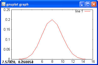
9.1.1  Discrete Distributions

Binomial

> x = 1:100;

> y = binopdf(x, 100, 0.5);

> plot(x, y)

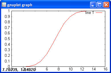
> y = binocdf(x, 100, 0.5)

> plot(x, y)

> x = 0:0.01:0.9;

> y = binoinv(x, 100, 0.5)

> plot(x, y)

> x = 1:5;

> y = binocdf(x, 10, 0.5);

> binoinv(y, 10, 0.5)

> ans =

1   2   3   4   5

> y = binornd(100, 0.5, 1, 10)

> y =

51   53   59   43   49   49   52   45   63   47

Geometric

> x = 1:10;

> y = geopdf(x, 0.5);

> plot(x, y);

> y = geocdf(x, 0.5)

> plot(x, y)

> y = geocdf(1:10, 0.5)

> x = geoinv(y, 0.5)

> x =

1   2   3   4   5   6   7   8   9   10

> geornd(0.05, 1, 5)

> ans =

2   16   21   0   190

Hypergeometric

> x = 0:15;

> y = hygepdf(x, 100, 40, 20);

> plot(x, y)

> y = hygecdf(x, 100, 40, 20)

> plot (x, y)

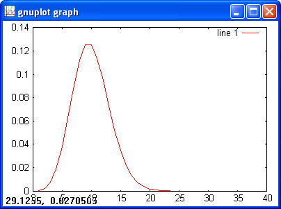
> x = 1:5;

> y = hygecdf(x, 100, 20, 10);

> hygeinv(y, 100, 20, 10)

> ans =

1   2   3   4   5

> hygernd(100,40,50)

> ans =

18

Poisson

> x = 1:40;

> y = poisspdf(x, 10);

> plot(x, y)

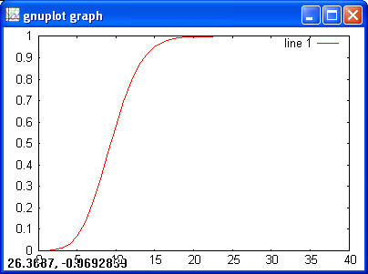
> y = poisscdf(x, 10)

> plot(x, y)

> x = 1:10;

> y = poisscdf(x, 3);

> poissinv(y, 3)

> ans =

1   2   3   4   5   6   7   8   9   10

> poissrnd(3, 1, 5)

> ans =

6   0   3   1   4

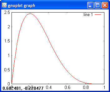
9.1.2 Continuous Distributions

Beta

> a = 2;

> b = 5;

> x = 0:0.01:1;

> y = betapdf(x, a, b);

> plot(x, y)

Other functions are not implemented at this point.

Chi-square

> x = 0:0.1:5;

> y = chi2pdf(x, 1);

> plot(x, y)

> y = chi2cdf(x, 1);

> plot(x, y)

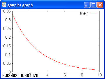
> chi2cdf(1, 1)

> ans =

0.6827

> chi2inv(0.6827, 1)

> ans =

1.0000

> chi2rnd(1, [2 3])

> ans =

Exponential

> x = 0:0.1:10;

> y = exppdf(x, 3);

> plot(x, y)

> y = expcdf(x, 3);

> plot (x, y)

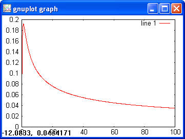
> x = 1:5;

> y = expcdf(x, 2);

> expinv(y, 2)

> ans =

1   2   3   4   5

F

> x = 0:0.1:100;

> y = fpdf(x, 2, 1);

> plot(x, y)

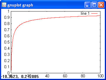
> y = fcdf(x, 2, 1)

> y = fcdf(1, 1, 10)

> ans =

0.6591

>finv(0.6591, 1, 10)

> ans =

1.0000

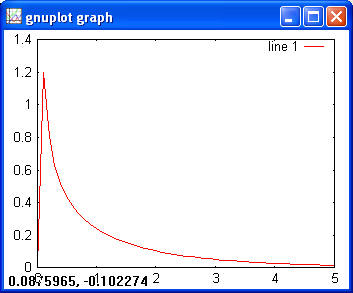
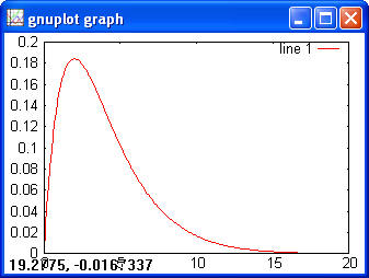
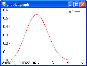
Gamma

> x = 0:0.1:20;

> y = gampdf(x, 2, 2);

> plot(x, y)

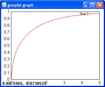
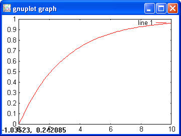
> y = gamcdf(x, 2, 2)

> plot(x, y)

> gamcdf(1, 2, 2)

> ans =

0.0902

> gaminv(0.0902, 2, 2)

> ans =

1.0000

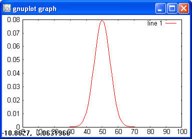
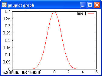
Normal

> x = -5:0.1:5;

> y = normpdf(x);

> plot(x, y)

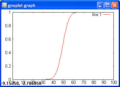
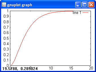
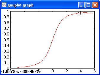
> y = normcdf(x)

> plot(x, y)

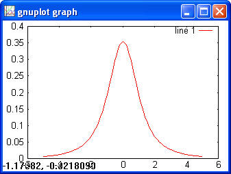
> normcdf(1)

> ans =

0.8413

> norminv(0.8413)

> ans =

0.9998

T

> x = -5:0.1:5;

> y = tpdf(x, 2);

> plot(x, y)

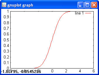
> y = tcdf(x, 2);

> plot(x, y)

> tcdf(1, 2)

> ans =

0.7887

> tinv(0.7887, 2)

> ans =

1.0001

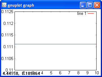
Uniform

> x = 1:10;

> y = unifpdf(x, 1, 10);

> plot(x, y)

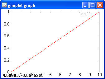
> y = unifcdf(x, 1, 10);

> plot(x, y)

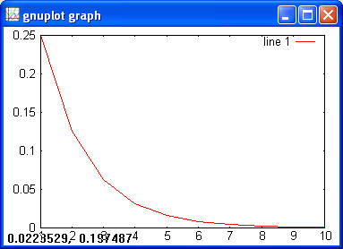
> unifcdf(2, 1, 10)

> ans =

0.1111

> unifinv(0.1111, 1, 10)

> ans =

1.9999

Weibull

> x = 0:0.1:5;

> y = weibpdf(x, 0.1, 3);

> plot(x, y)

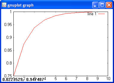
> y = weibcdf(x, 0.1, 3);

> plot(x, y)

> weibcdf(1, 1, 3)

> ans =

0.6321

> weibinv(0.6321, 1, 3)

> ans =

1.0000

9.2 Descriptive Statistics

numEclipse implements the following few functions for Descriptive statistics.

Mean

This method calculates the average value(s) for a matrix. The syntax is as follows

m = mean(X), or

m = mean(X, dim)

If X is a vector then "mean(X)" returns the mean value of X. In case of a matrix, it will return a row vector containing mean values of a corresponding columns in X.

"mean(X, dim)" allows to calculate mean along different dimensions of the matrix. For dim = 1, mean will be calculated along columns of X. For dim = 2, mean will be calculated along rows of X and the mean (X, dim) will return a column vector.

Example:

> x = [ 8 6 4; 0 4 9; 6 1 9];

> mean(x)

ans =

4.6667   3.6667   7.3333

> mean(x, 2)

ans =

6

4.3333

5.3333

Median

This method calculates the median value(s) for a matrix. The syntax is as follows

m = median(X), or

m = median(X, dim)

If X is a vector then "median(X)" returns the median value of X. In case of a matrix, it will return a row vector containing median values of a corresponding columns in X.

"median(X, dim)" allows to calculate median along different dimensions of the matrix. For dim = 1, median will be calculated along columns of X. For dim = 2, median will be calculated along rows of X and the median (X, dim) will return a column vector.

Example:

> x = [ 8 6 4; 0 4 9; 6 1 9];

> median(x)

ans =

6   4   9

> median(x, 2)

ans =

6

4

6

Var

This method calculates the variance value(s) for a matrix. The syntax is as follows

m = var(X), or

m = var(X, 1)

If X is a vector then "var(X)" returns the variance of X. In case of a matrix, it will return a row vector containing variance values of a corresponding columns in X.

"var" method normalizes by n-1 where n is the number of data values. Using "var(X, 1)", we can normalize by n.

Example:

> x = [ 8 6 4; 0 4 9; 6 1 9];

> var(x)

ans =

17.3333   6.3333   8.3333

> var(x, 1)

ans =

11.5556   4.2222   5.5556

std

This method calculates the standard deviation value(s) for a matrix. The syntax is as follows

m = std(X), or

m = std(X, 1)

If X is a vector then "std(X)" returns the standard deviation of X. In case of a matrix, it will return a row vector containing standard deviation values of a corresponding columns in X.

"std" method normalizes by n-1 where n is the number of data values. Using "std(X, 1)", we can normalize by n.

Example:

> x = [ 8 6 4; 0 4 9; 6 1 9];

> std(x)

ans =

4.1633   2.5166   2.8868

> std(x, 1)

ans =

3.3993   2.0548   2.3570

cov

This method calculates the covariance value(s) for a matrix. The syntax is as follows

m = cov(X), or

m = cov(X, Y)

"cov(X)" calculates the covariance matrix for X, where each column is considered as an observed values of a variable.

"cov(X,Y)" calculates the column-wise covariance between X and Y.

Example:

> x = [ 8 6 4; 0 4 9; 6 1 9];

> cov(x)

ans =

-2.0000   -4.0000   -5.6667

-5.0000   -1.0000    2.1667

5.0000    2.5000     -4.1667

9.3 Statistical Tests

numEclipse implements only two methods for statistical tests, i.e., t-test and z-test. These methods are adopted from octave.

t-test

Octave help provides following text.

Function File: [PVAL, T, DF] = ttest (X, M, ALT)
For a sample X from a normal distribution with unknown mean and
variance, perform a t-test of the null hypothesis `mean (X) == M'.
Under the null, the test statistic T follows a Student
distribution with `DF = length (X) - 1' degrees of freedom.

With the optional argument string ALT, the alternative of interest
can be selected. If ALT is `"!="' or `"<>"', the null is tested
against the two-sided alternative `mean (X) != M'. If ALT is
`">"', the one-sided alternative `mean (X) > M' is considered.
Similarly for "<", the one-sided alternative `mean (X) < M' is
considered, The default is the two-sided case.

The p-value of the test is returned in PVAL.
 

z-test

Octave help provides following text.

Function File: [PVAL, Z] = ztest (X, M, V, ALT)
Perform a Z-test of the null hypothesis `mean (X) == M' for a
sample X from a normal distribution with unknown mean and known
variance V. Under the null, the test statistic Z follows a
standard normal distribution.

With the optional argument string ALT, the alternative of interest
can be selected. If ALT is `"!="' or `"<>"', the null is tested
against the two-sided alternative `mean (X) != M'. If ALT is
`">"', the one-sided alternative `mean (X) > M' is considered.
Similarly for `"<"', the one-sided alternative `mean (X) < M' is
considered. The default is the two-sided case.
 

The p-value of the test is returned in PVAL.